机器学习-分类问题C

数学公式在渲染器中会出现错误，目前还没有解决

Outline

1. Nonlinear classifiers
2. Kernel trick and kernel SVM
3. Ensemble Methods - Boosting, Random Forests
4. Classification Summary

# setup
%matplotlib inline
import matplotlib_inline   # setup output image format
matplotlib_inline.backend_inline.set_matplotlib_formats('retina')
import matplotlib.pyplot as plt
plt.rcParams['figure.dpi'] = 100  # display larger images
import matplotlib
from numpy import *
from sklearn import *
from scipy import stats

def drawstump(fdim, fthresh, fdir='gt', poscol=None, negcol=None, lw=2, ls='k-'):
    # fdim = dimension
    # fthresh = threshold
    # fdir = direction (gt, lt)
    
    if fdir == 'lt':
        # swap colors
        tmp = poscol
        poscol = negcol
        negcol = tmp
    
    # assume fdim=0
    polyxn = [fthresh, fthresh, -30, -30]
    polyyn = [30, -30, -30, 30]
    
    polyxp = [fthresh, fthresh, 30, 30]
    polyyp = [30, -30, -30, 30]
        
    # fill positive half-space or neg space
    if (poscol):
        if fdim==0:
            plt.fill(polyxp, polyyp, poscol, alpha=0.2)
        else:
            plt.fill(polyyp, polyxp, poscol, alpha=0.2)            
    
    if (negcol):
        if fdim==0:
            plt.fill(polyxn, polyyn, negcol, alpha=0.2)
        else:
            plt.fill(polyyn, polyxn, negcol, alpha=0.2)

    # plot line
    if fdim==0:
        plt.plot(polyxp[0:2], polyyp[0:2], ls, lw=lw)
    else:
        plt.plot(polyyp[0:2], polyxp[0:2], ls, lw=lw)

def drawplane(w, b=None, c=None, wlabel=None, poscol=None, negcol=None, lw=2, ls='k-'):
    # w^Tx + b = 0
    # w0 x0 + w1 x1 + b = 0
    # x1 = -w0/w1 x0 - b / w1

    # OR
    # w^T (x-c) = 0 = w^Tx - w^Tc  --> b = -w^Tc
    if c != None:
        b = -sum(w*c)
    
    # the line
    if (abs(w[0])>abs(w[1])):   # vertical line
        x0 = array([-30,30])
        x1 = -w[0]/w[1] * x0 - b / w[1]
    else:                       # horizontal line
        x1 = array([-30,30])
        x0 = -w[1]/w[0] * x1 - b / w[0]
    
    # fill positive half-space or neg space
    if (poscol):
        polyx = [x0[0], x0[-1], x0[-1], x0[0]]
        polyy = [x1[0], x1[-1], x1[0], x1[0]]
        plt.fill(polyx, polyy, poscol, alpha=0.2)
    
    if (negcol):
        polyx = [x0[0], x0[-1], x0[0], x0[0]]
        polyy = [x1[0], x1[-1], x1[-1], x1[0]]
        plt.fill(polyx, polyy, negcol, alpha=0.2)
        
    # plot line
    lineplt, = plt.plot(x0, x1, ls, lw=lw)

    # the w
    if (wlabel):
        xp = array([0, -b/w[1]])
        xpw = xp+w
        plt.arrow(xp[0], xp[1], w[0], w[1], width=0.01)
        plt.text(xpw[0]-0.5, xpw[1], wlabel)
    return lineplt

# load iris data each row is (petal length, sepal width, class)
from sklearn.datasets import load_iris
from sklearn import model_selection

irisdata = load_iris()

X = irisdata.data[:100,0:2]  # the first two columns are features (petal length, sepal width)
Y = irisdata.target[:100]    # the third column is the class label (versicolor=1, virginica=2)

print(X.shape)

# randomly split data into 50% train and 50% test set
trainX, testX, trainY, testY = \
  model_selection.train_test_split(X, Y, 
  train_size=0.5, test_size=0.5, random_state=4487)

print(trainX.shape)
print(testX.shape)

(100, 2)
(50, 2)
(50, 2)

mycmap = matplotlib.colors.LinearSegmentedColormap.from_list('mycmap', ["#FF0000", "#FFFFFF", "#00FF00"])

axbox = [2.5, 7, 1.5, 4]

Feature Pre-processing

• Some classifiers, such as SVM and LR, are sensitive to the scale of the feature values.

  • feature dimensions with larger values may dominate the objective function.

• Common practice is to standardize or normalize each feature dimension before learning the classifier.

  • Two Methods…

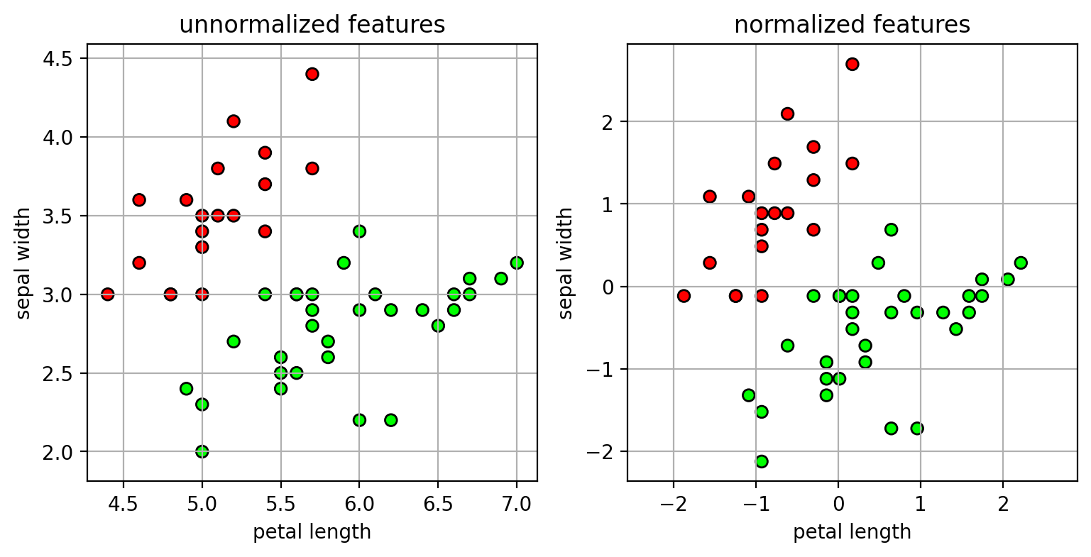
• Method 1: scale each feature dimension so the mean is 0 and variance is 1.

  • $\tilde{x}_d = \frac{1}{s}(x_d-m)$
  • $s$ is the standard deviation of feature values.
  • $m$ is the mean of the feature values.

• NOTE: the parameters for scaling the features should be estimated from the training set!

  • same scaling is applied to the test set.

# using the iris data
from sklearn import preprocessing
scaler = preprocessing.StandardScaler()  # make scaling object
trainXn = scaler.fit_transform(trainX)   # use training data to fit scaling parameters
testXn  = scaler.transform(testX)        # apply scaling to test data

nfig1 = plt.figure(figsize=(9,4))
axbox2 = [-3, 3, -3, 3]

plt.subplot(1,2,1)
plt.scatter(trainX[:,0], trainX[:,1], c=trainY, cmap=mycmap, edgecolors='k')
plt.xlabel('petal length'); plt.ylabel('sepal width')
plt.axis(axbox); plt.grid(True)
plt.axis('equal')
plt.title("unnormalized features")

plt.subplot(1,2,2)
plt.scatter(trainXn[:,0], trainXn[:,1], c=trainY, cmap=mycmap, edgecolors='k')
plt.xlabel('petal length'); plt.ylabel('sepal width')
plt.axis(axbox2); plt.grid(True)
plt.axis('equal')
plt.title("normalized features")
plt.close()

nfig1

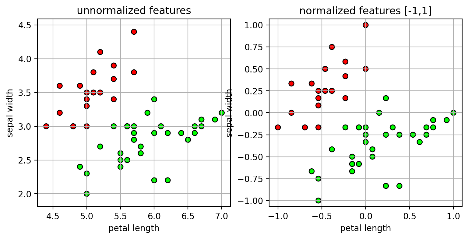
• Method 2: scale features to a fixed range, -1 to 1.
  • $\tilde{x}_d = 2*(x_d - min) / (max-min) - 1$
  • $max$ and $min$ are the maximum and minimum features values.

# using the iris data
scaler = preprocessing.MinMaxScaler(feature_range=(-1,1))    # make scaling object
trainXn = scaler.fit_transform(trainX)   # use training data to fit scaling parameters
testXn  = scaler.transform(testX)        # apply scaling to test data

nfig2 = plt.figure(figsize=(9,4))
axbox2 = [-1, 1, -1, 1]

plt.subplot(1,2,1)
plt.scatter(trainX[:,0], trainX[:,1], c=trainY, cmap=mycmap, edgecolors='k')
plt.xlabel('petal length'); plt.ylabel('sepal width')

plt.axis(axbox); plt.grid(True)
plt.axis('equal')
plt.title("unnormalized features")

plt.subplot(1,2,2)
plt.scatter(trainXn[:,0], trainXn[:,1], c=trainY, cmap=mycmap, edgecolors='k')
plt.xlabel('petal length'); plt.ylabel('sepal width')
plt.axis(axbox2); plt.grid(True)
plt.axis('equal')
plt.title("normalized features [-1,1]")
plt.close()

nfig2

Data Representation and Feature Engineering

• How to represent data as a vector of numbers?

  • the encoding of the data into a feature vector should make sense
  • inner-products or distances calculated between feature vectors should be meaningful in terms of the data.

• Categorical variables

  • Example: $x$ has 3 possible category labels: cat, dog, horse
  • We could encode this as: $x=0$, $x=1$, and $x=2$.
    • Suppose we have two data points: $x = cat$, $x’=horse$.
    • What is the meaning of $x*x’ = 2$?

One-hot encoding

• encode a categorical variable as a vector of ones and zeros
  • if there are $K$ categories, then the vector is $K$ dimensions.
• Example:
  • x=cat $\rightarrow$ x=[1 0 0]
  • x=dog $\rightarrow$ x=[0 1 0]
  • x=horse $\rightarrow$ x=[0 0 1]

# one-hot encoding example
X = [['cat'], ['dog'], ['cat'], ['bird'], ['dog']]  # each row is a sample
ohe = preprocessing.OneHotEncoder(sparse=False)
ohe.fit(X)         # map the categories to one-hot vectors
print(ohe.categories_)
ohe.transform(X)   # transform to one-hot-encoding

[array(['bird', 'cat', 'dog'], dtype=object)]


/Library/Frameworks/Python.framework/Versions/3.9/lib/python3.9/site-packages/sklearn/preprocessing/_encoders.py:828: FutureWarning: `sparse` was renamed to `sparse_output` in version 1.2 and will be removed in 1.4. `sparse_output` is ignored unless you leave `sparse` to its default value.
  warnings.warn(





array([[0., 1., 0.],
       [0., 0., 1.],
       [0., 1., 0.],
       [1., 0., 0.],
       [0., 0., 1.]])

Binning

• encode a real value as a vector of ones and zeros
  • assign each feature value to a bin, and then use one-hot-encoding

# example
X = [[-3], [0.5], [1.5], [2.5]]  # the data
bins = [-2,-1,0,1,2]      # define the bin edges

# map from value to bin number
Xbins = digitize(X, bins=bins)   

# map from bin number (0..5) to 0-1 vector
ohe = preprocessing.OneHotEncoder(categories=[arange(6)], sparse=False)
ohe.fit(Xbins)
ohe.transform(Xbins)

/Library/Frameworks/Python.framework/Versions/3.9/lib/python3.9/site-packages/sklearn/preprocessing/_encoders.py:828: FutureWarning: `sparse` was renamed to `sparse_output` in version 1.2 and will be removed in 1.4. `sparse_output` is ignored unless you leave `sparse` to its default value.
  warnings.warn(





array([[1., 0., 0., 0., 0., 0.],
       [0., 0., 0., 1., 0., 0.],
       [0., 0., 0., 0., 1., 0.],
       [0., 0., 0., 0., 0., 1.]])

Data transformations - polynomials

• Represent interactions between features using polynomials
• Example:
  • 2nd-degree polynomial models pair-wise interactions
    • $[x_1, x_2] \rightarrow [x_1^2, x_1 x_2, x_2^2]$
  • Combine with other degrees:
    • $[x_1, x_2] \rightarrow [1, x_1, x_2, x_1^2, x_1 x_2, x_2^2]$

X = [[0,1], [1,2], [3,4]]
pf = preprocessing.PolynomialFeatures(degree=2)
pf.fit(X)
pf.transform(X) 

array([[ 1.,  0.,  1.,  0.,  0.,  1.],
       [ 1.,  1.,  2.,  1.,  2.,  4.],
       [ 1.,  3.,  4.,  9., 12., 16.]])

Data transformations - univariate

• Apply a non-linear transformation to the feature
  • e.g., x $\rightarrow$ log(x)
  • useful if the dynamic range of x is very large

Unbalanced Data

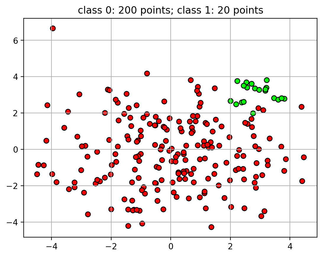
• For some classification tasks that data will be unbalanced
  • many more examples in one class than the other.
• Example: detecting credit card fraud
  • credit card fraud is rare
    • 50 examples of fraud, 5000 examples of legitimate transactions.

# generate random data
from sklearn import datasets
X,Y = datasets.make_blobs(n_samples=200, 
         centers=[[0,0]], cluster_std=2, n_features=2, random_state=4487)
X2,Y2 = datasets.make_blobs(n_samples=20, 
         centers=[[3,3]], cluster_std=0.5, n_features=2, random_state=4487)

X = r_[X,X2]
Y = r_[Y,Y2+1]

udatafig = plt.figure()
plt.scatter(X[:,0],X[:,1],c=Y,cmap=mycmap, edgecolors='k')
plt.grid(True)
plt.title('class 0: 200 points; class 1: 20 points')
plt.close()

udatafig

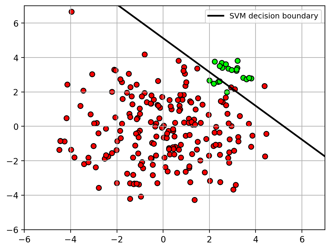
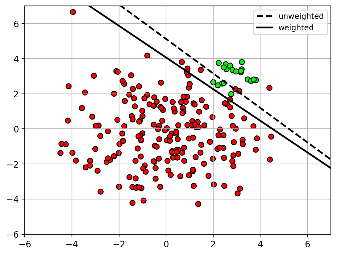
• Unbalanced data can cause problems when training the classifier
  • classifier will focus more on the class with more points.
  • decision boundary is pushed away from class with more points

from sklearn import svm
clf = svm.SVC(kernel='linear', C=10)
clf.fit(X, Y)

udatafig1 = plt.figure()
plt.scatter(X[:,0],X[:,1],c=Y,cmap=mycmap, edgecolors='k')

w = clf.coef_[0]
b = clf.intercept_[0]
l1 = drawplane(w, b, lw=2, ls='k-')
plt.legend((l1,), ('SVM decision boundary',), fontsize=9)
plt.axis([-6, 7, -6, 7])
plt.grid(True)
plt.close()

udatafig1

• Solution: apply weights on the classes during training.
  • weights are inversely proportional to the class size.

clfw = svm.SVC(kernel='linear', C=10,  class_weight='balanced')
clfw.fit(X, Y)

print("class weights =", clfw.class_weight_)

class weights = [0.55 5.5 ]

udatafig2 = plt.figure()
plt.scatter(X[:,0],X[:,1],c=Y,cmap=mycmap, edgecolors='k')

w = clf.coef_[0]
b = clf.intercept_[0]
ww = clfw.coef_[0]
bw = clfw.intercept_[0]
l1 = drawplane(w, b, lw=2, ls='k--')
l2 = drawplane(ww, bw, lw=2, ls='k-')
plt.legend((l1,l2), ('unweighted', 'weighted'), fontsize=9)
plt.axis([-6, 7, -6, 7])
plt.grid(True)
plt.close()

udatafig2

Classifier Imbalance

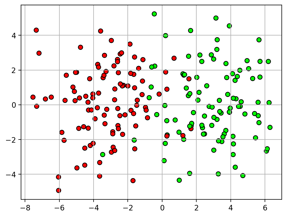
• In some tasks, errors on certain classes cannot be tolerated.
• Example: detecting spam vs non-spam
  • non-spam should definitely not be marked as spam
    • okay to mark some spam as non-spam

X,Y = datasets.make_blobs(n_samples=200, 
         centers=[[-3,0],[3,0]], cluster_std=2, n_features=2, random_state=447)
udatafig3 = plt.figure()
plt.scatter(X[:,0], X[:,1], c=Y, cmap=mycmap, edgecolors='k')
plt.grid(True)
plt.close()

clf = svm.SVC(kernel='linear', C=10)
clf.fit(X, Y)

SVC(C=10, kernel='linear')

In a Jupyter environment, please rerun this cell to show the HTML representation or trust the notebook.
On GitHub, the HTML representation is unable to render, please try loading this page with nbviewer.org.

udatafig3

…

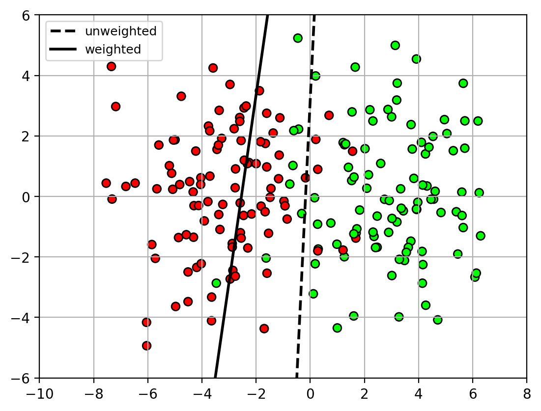
• Class weighting can be used to make the classifier focus on certain classes
  • e.g., weight non-spam class higher than spam class
    • classifier will try to correctly classify all non-spam samples, at the expense of making errors on spam samples.

# dictionary (key,value) = (class name, class weight)
cw = {0: 0.2, 
      1:  5}  # class 1 is 25 times more important!

clfw = svm.SVC(kernel='linear', C=10,  class_weight=cw)
clfw.fit(X, Y);

udatafig4 = plt.figure()
plt.scatter(X[:,0], X[:,1], c=Y, cmap=mycmap, edgecolors='k')
plt.grid(True)

w = clf.coef_[0]
b = clf.intercept_[0]
ww = clfw.coef_[0]
bw = clfw.intercept_[0]
l1 = drawplane(w, b, lw=2, ls='k--')
l2 = drawplane(ww, bw, lw=2, ls='k-')
plt.legend((l1,l2), ('unweighted', 'weighted'), fontsize=9)
plt.axis([-10, 8, -6, 6])

plt.close()

udatafig4

…

Classification Summary

• Classification task
  • Observation $\mathbf{x}$: typically a real vector of feature values, $\mathbf{x}\in\mathbb{R}^d$.
  • Class $y$: from a set of possible classes, e.g., ${\cal Y} = {0,1}$
  • Goal: given an observation $\mathbf{x}$, predict its class $y$.

Name	Type	Classes	Decision function	Training	Advantages	Disadvantages
Bayes' classifier	generative	multi-class	non-linear	estimate class-conditional densities $p(x|y)$ by maximizing likelihood of data.	- works well with small amounts of data. - multi-class. - minimum probability of error if probability models are correct.	- depends on the data correctly fitting the class-conditional.
logistic regression	discriminative	binary	linear	maximize likelihood of data in $p(y|x)$.	- well-calibrated probabilities. - efficient to learn.	- linear decision boundary. - sensitive to $C$ parameter.
support vector machine (SVM)	discriminative	binary	linear	maximize the margin (distance between decision surface and closest point).	- works well in high-dimension. - good generalization.	- linear decision boundary. - sensitive to $C$ parameter.
kernel SVM	discriminative	binary	non-linear (kernel function)	maximize the margin.	- non-linear decision boundary. - can be applied to non-vector data using appropriate kernel.	- sensitive to kernel function and hyperparameters. - high memory usage for large datasets
AdaBoost	discriminative	binary	non-linear (ensemble of weak learners)	train successive weak learners to focus on misclassified points.	- non-linear decision boundary. can do feature selection. - good generalization.	- sensitive to outliers.
XGBoost	discriminative	binary	non-linear (ensemble of decision trees)	train successive learners to focus on gradient of the loss.	- non-linear decision boundary. - good generalization.	- sensitive to outliers.
Random Forest	discriminative	multi-class	non-linear (ensemble of decision trees)	aggregate predictions over several decision trees, trained using different subsets of data.	- non-linear decision boundary. can do feature selection. - good generalization. - fast	- sensitive to outliers.

Loss functions

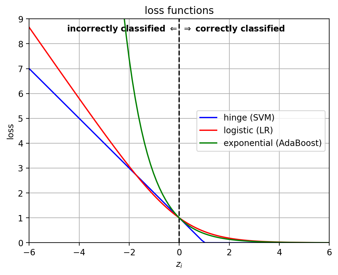
• The classifiers differ in their loss functions, which influence how they work.
  • $z_i = y_i f(\mathbf{x}_i)$

z = linspace(-6,6,100)
logloss = log(1+exp(-z)) / log(2)
hingeloss = maximum(0, 1-z)
exploss = exp(-z)
lossfig = plt.figure()

plt.plot([0,0], [0,9], 'k--')
plt.text(0,8.5, "incorrectly classified $\\Leftarrow$ ", ha='right', weight='bold')
plt.text(0,8.5, " $\Rightarrow$ correctly classified", ha='left', weight='bold')

plt.plot(z,hingeloss, 'b-', label='hinge (SVM)')
plt.plot(z,logloss, 'r-', label='logistic (LR)')
plt.plot(z,exploss, 'g-', label='exponential (AdaBoost)')
plt.axis([-6,6,0,9]); plt.grid(True)
plt.xlabel('$z_i$');
plt.ylabel('loss')
plt.legend(loc='right', fontsize=10)
plt.title('loss functions')
plt.close()

lossfig

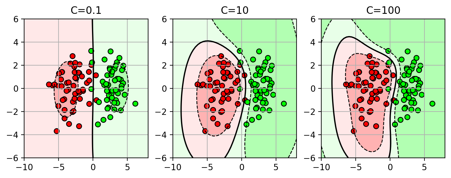
Regularization and Overfitting

• Some models have terms to prevent overfitting the training data.
  • this can improve generalization to new data.
• There is a parameter to control the regularization effect.
  • select this parameter using cross-validation on the training set.

X,Y = datasets.make_blobs(n_samples=100, 
         centers=[[-3,0],[3,0]], cluster_std=1.5, n_features=2, random_state=447)
udatafig3 = plt.figure()
axbox = [-10,8,-6,6]
xr = [linspace(axbox[0], axbox[1], 50), linspace(axbox[2], axbox[3], 50)]

Cs = [0.1, 10, 100]
clf={}

ofig = plt.figure(figsize=(9,3))
for i,C in enumerate(Cs):
    clf[C] = svm.SVC(kernel='rbf', C=C, gamma=0.05)
    clf[C].fit(X, Y)
    
    # make a grid for calculating the posterior, 
    #  then form into a big [N,2] matrix
    xgrid0, xgrid1 = meshgrid(xr[0], xr[1])
    allpts = c_[xgrid0.ravel(), xgrid1.ravel()]

    score = clf[C].decision_function(allpts).reshape(xgrid0.shape)

    cmap = ([1,0,0], [1,0.7,0.7], [0.7,1,0.7], [0,1,0])
    
    plt.subplot(1,len(Cs),i+1)
    plt.contourf(xr[0], xr[1], score, colors=cmap, 
             levels=[-1000, -1, 0, 1, 1000], alpha=0.3)
    plt.contour(xr[0], xr[1], score, levels=[-1, 1], linewidths=1, linestyles='dashed', colors='k')
    plt.contour(xr[0], xr[1], score, levels=[0], linestyles='solid', colors='k')

    plt.scatter(X[:,0], X[:,1], c=Y, cmap=mycmap, edgecolors='k')
    
    #plt.plot(clf.support_vectors_[:,0], clf.support_vectors_[:,1],
    #         'ko',fillstyle='none', markeredgewidth=2)
    plt.axis(axbox); plt.grid(True)
    plt.title('C='+str(C))
plt.close()

<Figure size 640x480 with 0 Axes>

ofig

​

​

Structural Risk Minimization

• A general framework for balancing data fit and model complexity.
• Many learning problems can be written as a combination of data-fit and regularization term:
  $$f^* = \mathop{\mathrm{argmin}}_{f} \sum_i L(y_i, f(\mathbf{x}_i)) + \lambda \Omega(f)$$
  • assume $f$ within some class of funcitions, e.g., linear functions $f(\mathbf{x}) = \mathbf{w}^T\mathbf{x}+b$.
  • $L$ is the loss function, e.g., logistic loss.
  • $\Omega$ is the regularization function on $f$, e.g., $||\mathbf{w}||^2$
  • $\lambda$ is the tradeoff parameter, e.g., $1/C$.

Other things

• Multiclass classification
  • can use binary classifiers to do multi-class using 1-vs-rest formulation.
• Feature normalization
  • normalize each feature dimension so that some feature dimensions with larger ranges do not dominate the optimization process.
• Unbalanced data
  • if more data in one class, then apply weights to each class to balance objectives.
• Class imbalance
  • mistakes on some classes are more critical.
  • reweight class to focus classifier on correctly predicting one class at the expense of others.

Applications

• Web document classification, spam classification
• Face gender recognition, face detection, digit classification

Features

• Choice of features is important!
  • using uninformative features may confuse the classifier.
  • use domain knowledge to pick the best features to extract from the data.

Which classifier is best?

• “No Free Lunch” Theorem (Wolpert and Macready)

“If an algorithm performs well on a certain class of problems then it necessarily pays for that with degraded performance on the set of all remaining problems.”

• In other words, there is no best classifier for all tasks. The best classifier depends on the particular problem.