机器学习-分类问题A

数学公式在渲染器中会出现错误,目前还没有解决

Outline

  1. Nonlinear classifiers
  2. Kernel trick and kernel SVM
  3. Ensemble Methods - Boosting, Random Forests
  4. Classification Summary
1
2
3
4
5
6
7
8
9
10
# setup
%matplotlib inline
import matplotlib_inline # setup output image format
matplotlib_inline.backend_inline.set_matplotlib_formats('retina')
import matplotlib.pyplot as plt
plt.rcParams['figure.dpi'] = 100 # display larger images
import matplotlib
from numpy import *
from sklearn import *
from scipy import stats
1
2
3
4
5
6
7
8
9
10
11
12
13
14
15
16
17
18
19
20
21
22
23
24
25
26
27
28
29
30
31
32
33
34
35
36
37
38
39
40
41
42
43
44
45
46
47
48
49
50
51
52
53
54
55
56
57
58
59
60
61
62
63
64
65
66
67
68
69
70
def drawplane(w, b=None, c=None, wlabel=None, poscol=None, negcol=None, lw=2, ls='k-', label=None):
# w^Tx + b = 0
# w0 x0 + w1 x1 + b = 0
# x1 = -w0/w1 x0 - b / w1

# OR
# w^T (x-c) = 0 = w^Tx - w^Tc --> b = -w^Tc
if c is not None:
b = -sum(w*c)

# the line
if (abs(w[0])>abs(w[1])): # vertical line
x0 = array([-30,30])
x1 = -w[0]/w[1] * x0 - b / w[1]
else: # horizontal line
x1 = array([-30,30])
x0 = -w[1]/w[0] * x1 - b / w[0]

# fill positive half-space or neg space
if (poscol):
polyx = [x0[0], x0[-1], x0[-1], x0[0]]
polyy = [x1[0], x1[-1], x1[0], x1[0]]
plt.fill(polyx, polyy, poscol, alpha=0.2)

if (negcol):
polyx = [x0[0], x0[-1], x0[0], x0[0]]
polyy = [x1[0], x1[-1], x1[-1], x1[0]]
plt.fill(polyx, polyy, negcol, alpha=0.2)

# plot line
plt.plot(x0, x1, ls, lw=lw, label=label)

# the w
if (wlabel):
xp = array([0, -b/w[1]])
xpw = xp+w
plt.arrow(xp[0], xp[1], w[0], w[1], width=0.01)
plt.text(xpw[0]-0.5, xpw[1], wlabel)

def drawmargin(w,b,xmarg=None, label=None):
wnorm = w / sqrt(sum(w**2))
if xmarg is None:
# calculate a point on the margin
dm = 1 / sqrt(sum(w**2))
xpt = array([1,-w[0]/w[1]-b/w[1]])
# then find the margin (assuming learned with SVM)
xmarg = xpt + dm*wnorm
xmarg2 = xpt - dm*wnorm
else:
# find the distance to the margin
dm = (sum(w*xmarg)+b) / sqrt(sum(w**2))
# move to the other side of the decision plane
xmarg2 = xmarg - 2*dm*wnorm

drawplane(w, c=xmarg, ls='k--', lw=1, label=label)
drawplane(w, c=xmarg2, ls='k--', lw=1)

def plot_svm(clf, axbox, mycmap, showleg=True):
# get line parameters
w = clf.coef_[0]
b = clf.intercept_[0]

drawplane(w, b, poscol='g', negcol='r', label='boundary')
drawmargin(w, b, label='margin')
plt.plot(clf.support_vectors_[:,0], clf.support_vectors_[:,1],
'ko',fillstyle='none', markeredgewidth=2, label='support vectors')
plt.axis(axbox); plt.grid(True)
if showleg:
leg = plt.legend(loc='lower right', fontsize=10)
leg.get_frame().set_facecolor('white')

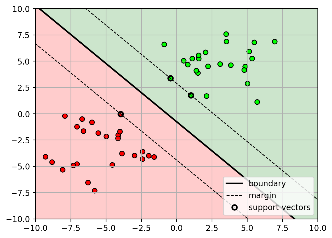
Linear Classifiers

  • So far we have only looked at linear classifiers
    • separate classes using a hyperplane (line, plane).
    • e.g., support vector machine, logistic regression
1
2
3
4
5
6
7
8
9
10
11
12
13
14
15
16
17
18
# generate random data
from sklearn import datasets
from sklearn import svm
X,Y = datasets.make_blobs(n_samples=50,
centers=2, cluster_std=2, n_features=2,
center_box=[-5,5], random_state=4487)
mycmap = matplotlib.colors.LinearSegmentedColormap.from_list('mycmap', ["#FF0000", "#FFFFFF", "#00FF00"])

axbox = [-10,10,-10,10]

# fit SVM (kernel is the type of decision surface...more in the next lecture)
clf = svm.SVC(kernel='linear', C=1)
clf.fit(X, Y)

maxmfig = plt.figure()
plot_svm(clf, axbox, mycmap)
plt.scatter(X[:,0], X[:,1], c=Y, cmap=mycmap, edgecolors='k')
plt.close()
1
maxmfig

png

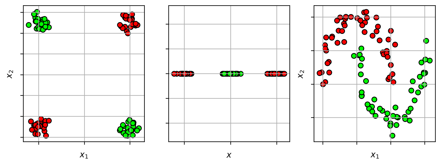
Non-linear decision boundary

  • What if the data is separable, but not linearly separable?
1
2
3
4
5
6
7
8
9
10
11
12
13
14
15
16
17
18
19
20
21
22
23
24
25
26
27
28
29
30
31
32
33
nlfig = plt.figure(figsize=(9,3))
plt.subplot(1,3,1)
# type one - XOR
X1,Y1 = datasets.make_blobs(n_samples=100,
centers=array([[5,5],[-5,-5],[-5, 5], [5, -5]]), cluster_std=0.5, n_features=2,
random_state=4487)
Y1 = (Y1>=2)+0
plt.scatter(X1[:,0], X1[:,1], c=Y1, cmap=mycmap, edgecolors='k')
plt.xlabel('$x_1$'); plt.ylabel('$x_2$'); plt.grid(True)
plt.gca().xaxis.set_ticklabels([])
plt.gca().yaxis.set_ticklabels([])

# type two - split
X2,Y2 = datasets.make_blobs(n_samples=100,
centers=array([[5],[-5],[0]]), cluster_std=0.5, n_features=1,
random_state=4487)
Y2 = (Y2>1)+0
plt.subplot(1,3,2)
plt.scatter(X2[:,0], zeros(X2.shape), c=Y2, cmap=mycmap, edgecolors='k')
plt.xlabel('$x$'); plt.grid(True)
plt.gca().xaxis.set_ticklabels([])
plt.gca().yaxis.set_ticklabels([])


# type three - moons
X3,Y3 = datasets.make_moons(n_samples=100,
noise=0.1, random_state=4487)
plt.subplot(1,3,3)
plt.scatter(X3[:,0], X3[:,1], c=Y3, cmap=mycmap, edgecolors='k')
plt.xlabel('$x_1$'); plt.ylabel('$x_2$'); plt.grid(True)
plt.gca().xaxis.set_ticklabels([])
plt.gca().yaxis.set_ticklabels([])
plt.close()
1
nlfig

png

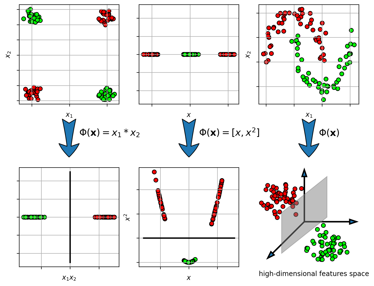
Idea - transform the input space

  • map from input space $\mathbf{x} \in \mathbb{R}^d$ to a new high-dimensional space $\mathbf{z} \in \mathbb{R}^D$.
    • $\mathbf{z} = \Phi(\mathbf{x})$, where $\Phi(\mathbf{x})$ is the transformation function.
  • learn the linear classifier in the new space
    • if dimension of new space is large enough ($D>d$), then the data should be linearly separable
1
2
3
4
5
6
7
8
9
10
11
12
13
14
15
16
17
18
19
20
21
22
23
24
25
26
27
28
29
30
31
32
33
34
35
36
37
38
39
40
41
42
43
44
45
46
47
48
49
50
51
52
53
54
55
56
57
58
59
60
61
62
63
64
65
66
67
68
69
70
71
72
73
74
75
76
77
78
nl2fig = plt.figure(figsize=(9,7))

# type one - XOR
plt.subplot2grid((5,3),(0,0), rowspan=2)
plt.scatter(X1[:,0], X1[:,1], c=Y1, cmap=mycmap, edgecolors='k')
plt.xlabel('$x_1$'); plt.ylabel('$x_2$'); plt.grid(True)
plt.gca().xaxis.set_ticklabels([])
plt.gca().yaxis.set_ticklabels([])

X1t = X1[:,0]*X1[:,1]

plt.subplot2grid((5,3),(2,0))
plt.annotate("", xy=(0, -1), xytext=(0,0.8),
arrowprops=dict(arrowstyle='Fancy,head_width=3,tail_width=2,head_length=2'))
plt.text(0.2,0,"$\Phi(\mathbf{x}) = x_1*x_2$", fontsize=14)
plt.axis([-1, 1, -1, 1])
plt.axis('off')

plt.subplot2grid((5,3),(3,0), rowspan=2)
plt.scatter(X1t, zeros(X1t.shape), c=Y1, cmap=mycmap, edgecolors='k')
plt.xlabel('$x_1 x_2$'); plt.grid(True)
plt.gca().xaxis.set_ticklabels([])
plt.gca().yaxis.set_ticklabels([])
plt.plot([0,0],[-0.5,0.5], 'k-', lw=2)

# type two - split
plt.subplot2grid((5,3),(0,1), rowspan=2)
plt.scatter(X2[:,0], zeros(X2.shape), c=Y2, cmap=mycmap, edgecolors='k')
plt.xlabel('$x$'); plt.grid(True)
plt.gca().xaxis.set_ticklabels([])
plt.gca().yaxis.set_ticklabels([])


plt.subplot2grid((5,3),(2,1))
plt.annotate("", xy=(0, -1), xytext=(0,0.8),
arrowprops=dict(arrowstyle='Fancy,head_width=3,tail_width=2,head_length=2'))
plt.text(0.2,0,"$\Phi(\mathbf{x}) = [x, x^2]$", fontsize=14)
plt.axis([-1, 1, -1, 1])
plt.axis('off')


X2t = c_[X2, X2**2]
plt.subplot2grid((5,3),(3,1), rowspan=2)
plt.scatter(X2t[:,0], X2t[:,1], c=Y2, cmap=mycmap, edgecolors='k')
plt.xlabel('$x$'); plt.ylabel('$x^2$');plt.grid(True)
plt.plot([-8,8],[10,10], 'k-', lw=2)
plt.gca().xaxis.set_ticklabels([])
plt.gca().yaxis.set_ticklabels([])

# type three - moons
plt.subplot2grid((5,3),(0,2), rowspan=2)
plt.scatter(X3[:,0], X3[:,1], c=Y3, cmap=mycmap, edgecolors='k')
plt.xlabel('$x_1$'); plt.ylabel('$x_2$'); plt.grid(True)
plt.gca().xaxis.set_ticklabels([])
plt.gca().yaxis.set_ticklabels([])

plt.subplot2grid((5,3),(2,2))
plt.annotate("", xy=(0, -1), xytext=(0,0.8),
arrowprops=dict(arrowstyle='Fancy,head_width=3,tail_width=2,head_length=2'))
plt.text(0.2,0,"$\Phi(\mathbf{x})$", fontsize=14)
plt.axis([-1, 1, -1, 1])
plt.axis('off')

plt.subplot2grid((5,3),(3,2), rowspan=2)
plt.arrow(0,0, 10,0, lw=2, head_width=1)
plt.arrow(0,0, 0,10, lw=2, head_width=1)
plt.arrow(0,0, -7,-7, lw=2, head_width=1)

X3t,Y3t = datasets.make_blobs(n_samples=100,
centers=array([[-5,5],[5,-5]]), cluster_std=2, n_features=2,
random_state=4487)
plt.scatter(X3t[:,0], X3t[:,1], c=Y3t, cmap=mycmap, edgecolors='k')
plt.fill([5, -5, -5, 5], [10, 2, -7, 1], alpha=0.5, color='gray', ls='solid')
plt.axis([-10, 12, -10, 12])
plt.text(-10,-12,"high-dimensional features space")
plt.axis('off')

plt.close()
1
nl2fig

png

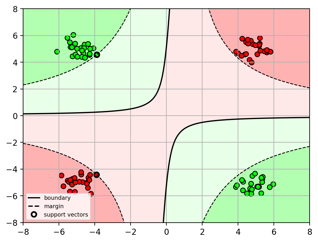
Example

  • Let’s try it…
    - 2-dimensional vector inputs

    $$
    \mathbf{x} = \begin{bmatrix}x_1\\x_2\end{bmatrix}
    $$
    
    • transformation consists of quadratic terms

      $$
      \Phi(\mathbf{x}) = \begin{bmatrix} x_1^2 \ x_1x_2 \ x_2^2 \end{bmatrix}
      $$
1
2
3
4
5
6
7
8
9
10
11
12
13
14
15
16
17
18
19
20
21
22
23
24
25
26
27
28
29
30
31
32
33
34
35
def plot_posterior_svm(model, axbox, X, phi=None):
# grid points
xr = [ linspace(axbox[0], axbox[1], 200),
linspace(axbox[2], axbox[3], 200) ]

# make a grid for calculating the posterior,
# then form into a big [N,2] matrix
xgrid0, xgrid1 = meshgrid(xr[0], xr[1])
allptsx = c_[xgrid0.ravel(), xgrid1.ravel()]

# transform
if phi != None:
allpts = apply_along_axis(phi, 1, allptsx)
else:
allpts = allptsx

# calculate the score
score = model.decision_function(allpts).reshape(xgrid0.shape)

cmap = ([1,0,0], [1,0.7,0.7], [0.7,1,0.7], [0,1,0])
CS = plt.contourf(xr[0], xr[1], score, colors=cmap,
levels=[-1000, -1, 0, 1, 1000], alpha=0.3)

plt.contour(xr[0], xr[1], score, levels=[-1, 1], linewidths=1, linestyles='dashed', colors='k')
plt.contour(xr[0], xr[1], score, levels=[0], linestyles='solid', colors='k')

plt.plot([-100,-100], [-100,-100], 'k-', label='boundary')
plt.plot([-100,-100], [-100,-100], 'k--', label='margin')

plt.plot(X[model.support_,0], X[model.support_,1],
'ko',fillstyle='none', markeredgewidth=2, label='support vectors')

leg = plt.legend(loc='best', fontsize=7)
leg.get_frame().set_facecolor('white')
plt.axis(axbox); plt.grid(True)
1
2
3
4
5
6
7
8
9
10
# define the transformation function for a vector x
# (a lambda function is an anonymous function)
phi = lambda x: array([x[0]**2, x[1]**2, x[0]*x[1]])

# apply function phi to each row of data matrix X1
PX = apply_along_axis(phi, 1, X1)

# fit SVM with transformed data
clf = svm.SVC(kernel='linear', C=1)
clf.fit(PX, Y1)
SVC(C=1, kernel='linear')
In a Jupyter environment, please rerun this cell to show the HTML representation or trust the notebook.
On GitHub, the HTML representation is unable to render, please try loading this page with nbviewer.org.
1
2
3
4
5
# make plot
axbox = [-8, 8, -8, 8]
plt.figure()
plot_posterior_svm(clf, axbox, X1, phi=phi)
plt.scatter(X1[:,0], X1[:,1], c=Y1, cmap=mycmap, edgecolors='k');

png

SVM with transformed input

  • Given a training set
    $$
    {\mathbf{x}i,y_i}{i=1}^N
    $$
    ,

  • the original SVM training is:
    $$ \mathop{\mathrm{argmin}}_{\mathbf{w},b} \frac{1}{2} \mathbf{w}^T\mathbf{w}\quad \mathrm{s.t.}~y_i (\mathbf{w}^T\mathbf{x}_i+b)\geq 1,\quad 1\leq i \leq N$$

  • Apply high-dimensional transform to input $$\mathbf{x}\rightarrow \Phi(\mathbf{x})$$:
    $$ \mathop{\mathrm{argmin}}_{\mathbf{w},b} \frac{1}{2} \mathbf{w}^T\mathbf{w}\quad \mathrm{s.t.}~y_i(\mathbf{w}^T\Phi(\mathbf{x}_i)+b)\geq 1,\quad 1\leq i \leq N$$

  • Note: the hyperplane $$\mathbf{w}\in\mathbb{R}^D$$ is now in the high-dimensional space!

    • if $D$ is very large,
      • calculating feature vector $\Phi(\mathbf{x}_i)$ could be time consuming.
      • optimization could be very inefficient in high-dimensional space.
    • To solve this problem requires some optimization theory…

Review of Constrained Optimization

  • Consider an optimization problem with inequality constraints:
    $$ \min_{\mathbf{x}} f(\mathbf{x})\ \text{s.t.}\ g(\mathbf{x}) \geq 0$$
    • $f(\mathbf{x})$ is the objective function (for SVM, it’s the inverse margin).
    • $g(\mathbf{x})$ is the constraint function (for SVM, it’s the margin constraint).
  • Use Langrange multipliers to solve this problem:
    • introduce Lagrange multiplier: $\lambda \geq 0$
    • form the Lagrangian: $L(\mathbf{x},\lambda) = f(\mathbf{x}) - \lambda g(\mathbf{x})$
    • find the stationary point $(\mathbf{x}^*, \lambda^*)$ of the Lagrangian
      • find solution of $\frac{dL}{d\mathbf{x}}=0$ and $\frac{dL}{d\lambda}=0$.
    • at the solution, the Langrange multiplier indicates the mode of the inequality constraint
      • when $\lambda^*>0$, then $g(\mathbf{x}^*)=0$ (called “active equality”).
      • when $\lambda^*=0$, then $g(\mathbf{x}^*)>0$ (called “inactive”).

Duality

  • We can rewrite the original (primal) problem into its dual form:

    • dual function: $q(\lambda) = \min_{\mathbf{x}} L(\mathbf{x},\lambda)$
    • dual problem: $\max_{\lambda\geq 0} q(\lambda)$
  • Solve for $\lambda$, rather than original variable $\mathbf{x}$.

    • can recover the value of $\mathbf{x}$ from $\lambda$.
  • If the optimization problem is convex…

    • solving the dual is equivalent to solving the primal
    • $\min_{\mathbf{x}, g(\mathbf{x})\geq 0} f(\mathbf{x}) = \max_{\lambda\geq 0} q(\lambda)$.
  • Note: The SVM problem is convex, so we can obtain an equivalent dual problem.

Lagrange multipliers & SVM

  • introduce a Langrange multiplier $\alpha_i$ for each constrain
    $$ L(\mathbf{w}, \alpha) = \frac{1}{2} \mathbf{w}^T\mathbf{w}- \sum_i \alpha_i [y_i(\mathbf{w}^T\mathbf{x}_i+b)-1] $$
  • Lagrange multiplier tells us which points are on the margin:
    • If $\alpha_i=0$, then $y_i(\mathbf{w}^T\mathbf{x}_i+b)>1$ ($\mathbf{x}_i$ is beyond margin).
    • If $\alpha_i>0$, then $y_i(\mathbf{w}^T\mathbf{x}_i+b)=1$ ($\mathbf{x}_i$ is on the margin).
      • i.e., the point is a support vector.

SVM Dual Problem

  • The SVM problem can be rewritten as a dual problem:
    $$
    \mathop{\mathrm{argmax}}{\alpha} \sum_i \alpha_i -\frac{1}{2}\sum{i=1}^N\sum_{j=1}^N \alpha_i\alpha_j y_i y_j \Phi(\mathbf{x}_i)^T \Phi(\mathbf{x}j) \ \mathrm{s.t.} \sum{i=1}^N \alpha_iy_i = 0, \quad \alpha_i\geq 0
    $$

  • The new variable $\alpha_i$ corresponds to each training sample $(\mathbf{x}_i,y_i)$.

    • instead of solving for $\mathbf{w}$, we now solve for $\mathbf{\alpha}$
  • For soft-margin SVM, the constraint on $\alpha$ is $C\geq \alpha_i\geq 0$

  • Recover the hyperplane $\mathbf{w}$ using $\alpha$:

    • weighted combination of (transformed) data points.
    • $\mathbf{w} = \sum_{i=1}^N \alpha_i y_i \Phi(\mathbf{x}_i)$
  • Classify a new point $\mathbf{x}*$,
    $$\begin{align}y
    * &= \mathrm{sign}(\mathbf{w}^T\Phi(\mathbf{x}*)+b) \&= \mathrm{sign}(\sum{i=1}^N \alpha_i y_i \Phi(\mathbf{x}i)^T \Phi(\mathbf{x}*) + b)\end{align}$$

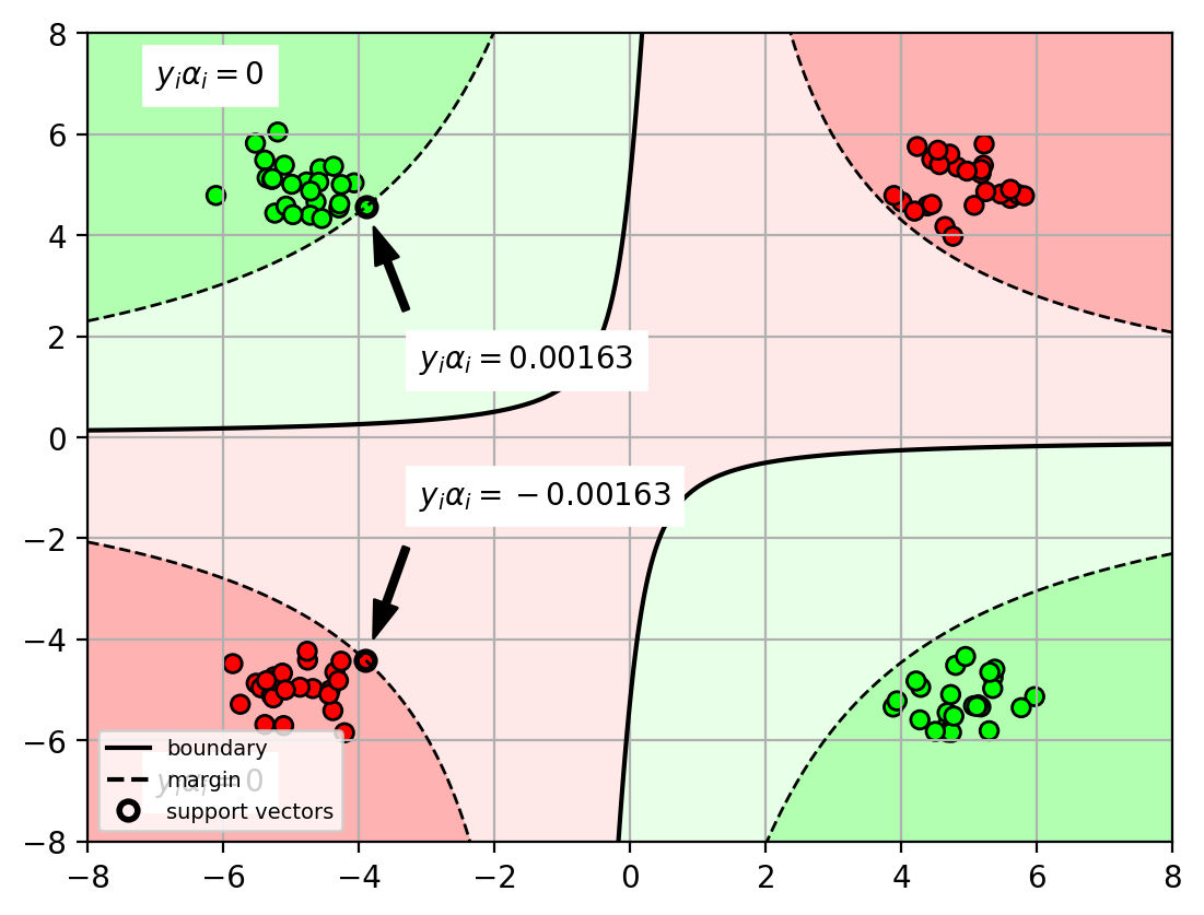
  • Interpretation of $\alpha_i$

    • $\alpha_i=0$ when the sample $\mathbf{x}_i$ is not on the margin.
    • $\alpha_i>0$ when the sample $\mathbf{x}_i$ is on the margin (or violates).
      • i.e., the sample $\mathbf{x}_i$ is a support vector.
      • $y_i\alpha_i > 0$ margin sample for positive class
      • $y_i\alpha_i < 0$ margin sample for negative class.
1
2
3
4
5
6
7
8
9
10
11
12
13
alfig = plt.figure()
plot_posterior_svm(clf, axbox, X1, phi=phi)
plt.scatter(X1[:,0], X1[:,1], c=Y1, cmap=mycmap, edgecolors='k')
for i,s in enumerate(clf.support_):
myal = clf.dual_coef_[0][i]
myx = X1[s]
plt.annotate("$y_i\\alpha_i=%0.3g$" % myal, xy=myx, xytext=(myx)*(0.8, 0.3),
arrowprops=dict(facecolor='black', shrink=0.15, width=2, headwidth=8),
backgroundcolor='white',
)
plt.text(-7,7,"$y_i\\alpha_i=0$", backgroundcolor='white')
plt.text(-7,-7,"$y_i\\alpha_i=0$", backgroundcolor='white')
plt.close()
1
alfig

png

Kernel function

  • the SVM dual problem is completely written in terms of inner product between the high-dimensional feature vectors: $\Phi(\mathbf{x}_i)^T \Phi(\mathbf{x}_j)$
  • So rather than explicitly calculate the high-dimensional vector $\Phi(\mathbf{x}_i)$,
    • we only need to calculate the inner product between two high-dim feature vectors.
  • We call this a kernel function
    • $k(\mathbf{x}_i, \mathbf{x}_j) = \Phi(\mathbf{x}_i)^T \Phi(\mathbf{x}_j)$
    • calculating the kernel will be less expensive than explicitly calculating the high-dimensional feature vector and the inner product.

Example: Polynomial kernel

  • input vector $
    $$
    \mathbf{x}=\left[\begin{matrix}x_1\\vdots\x_d\end{matrix}\right]\in\mathbb{R}^d
    $$
    $

  • kernel between two vectors is a $p$-th order polynomial:

    • $k(\mathbf{x},\mathbf{x}’) = (\mathbf{x}^T\mathbf{x}’)^p = (\sum_{i=1}^d x_i x_i’)^p$
  • For example, $p=2$,
    $$\begin{align}k(\mathbf{x},\mathbf{x}’) &= (\mathbf{x}^T \mathbf{x}’)^2 = (\sum_{i=1}^d x_i x_i’)^2 \ &= \sum_{i=1}^d \sum_{j=1}^d (x_ix_i’ x_jx_j’) = \Phi(\mathbf{x})^T \Phi(\mathbf{x}’)\end{align}$$

    • transformed feature space is the quadratic terms of the input vector:
      $$
      \Phi(\mathbf{x}) = \left[\begin{matrix} x_1 x_1 \ x_1 x_2 \ \vdots \
      x_2 x_1 \x_2 x_2 \ \vdots \
      x_d x_1 \ \vdots \ x_d x_d
      \end{matrix}\right]
      $$
  • Comparison of number of multiplications

    • for kernel: $O(d)$
    • explicit transformation $\Phi$: $O(d^2)$

Kernel trick

  • Replacing the inner product with a kernel function in the optimization problem is called the kernel trick.
    • turns a linear classification algorithm into a non-linear classification algorithm.
    • the shape of the decision boundary is determined by the kernel.

Kernel SVM

  • Replace inner product in linear SVM with kernel function:
    $$
    \mathop{\mathrm{argmax}}{\alpha} \sum_i \alpha_i -\frac{1}{2}\sum{i=1}^N\sum_{j=1}^N \alpha_i\alpha_j y_i y_j k(\mathbf{x}_i, \mathbf{x}j) \ \mathrm{s.t.} \sum{i=1}^N \alpha_iy_i = 0, \quad \alpha_i\geq 0
    $$

  • Prediction

    $$
    y_* = \mathrm{sign}(\sum_{i=1}^N \alpha_i y_i k(\mathbf{x}i, \mathbf{x}*) + b)
    $$

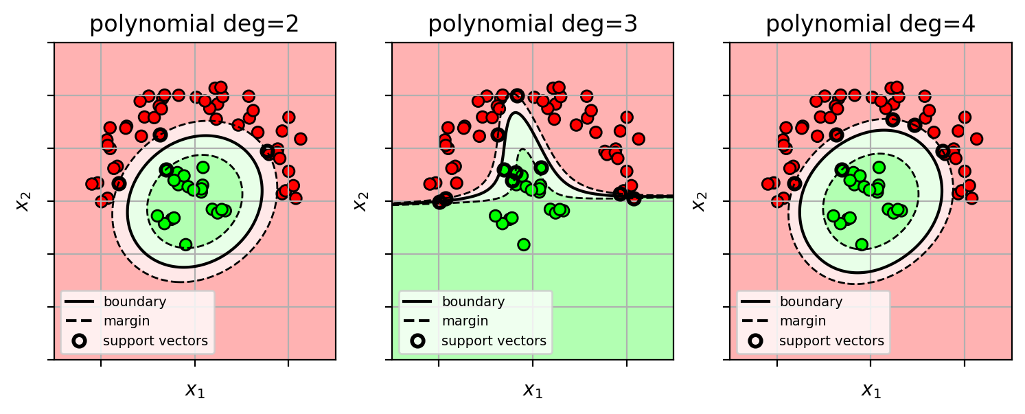
Example: Kernel SVM with polynomial kernel

  • decision surface is a “cut” of a polynomial surface
  • higher polynomial-order yields more complex decision boundaries.
1
2
3
4
5
6
7
8
inds = (Y3==0)
X4 = X3[inds]
Y4 = Y3[inds]
tmpX,tmpY = datasets.make_blobs(n_samples=20,
centers=1, cluster_std=0.2, n_features=2,
center_box=[0,0], random_state=4487)
X4 = vstack((X4,tmpX))
Y4 = r_[Y4, tmpY+1]
1
2
3
4
5
6
7
# fit SVM (poly kernel with different degrees)
degs = [2,3,4]

clf = {}
for d in degs:
clf[d] = svm.SVC(kernel='poly', degree=d, C=100)
clf[d].fit(X4, Y4)
1
2
3
4
5
6
7
8
9
10
11
12
13
axbox = [-1.5, 1.5, -1.5, 1.5]

polysvmfig = plt.figure(figsize=(9,3))

for (i,d) in enumerate(degs):
plt.subplot(1,3,i+1)
plot_posterior_svm(clf[d], axbox, X4)
plt.scatter(X4[:,0], X4[:,1], c=Y4, cmap=mycmap, edgecolors='k')
plt.xlabel('$x_1$'); plt.ylabel('$x_2$')
plt.gca().xaxis.set_ticklabels([])
plt.gca().yaxis.set_ticklabels([])
plt.title('polynomial deg=' + str(degs[i]))
plt.close()
1
polysvmfig

png

RBF kernel

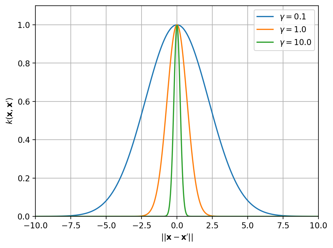
  • RBF kernel (radial basis function)
    • $k(\mathbf{x},\mathbf{x}’) = e^{-\gamma|\mathbf{x}-\mathbf{x}’|^2}$
    • similar to a Gaussian
  • gamma $\gamma>0$ is the inverse bandwidth parameter of the kernel
    • controls the smoothness of the function
    • small $\gamma$ -> wider RBF -> smooth functions
    • large $\gamma$ -> thin RBF -> wiggly function
1
2
3
4
5
6
7
8
9
10
11
rbffig = plt.figure()
x = linspace(-10,10,500)
gammas = array([0.1, 1.0, 10.0])
for g in gammas:
kx = exp(-g*(x**2))
plt.plot(x, kx, label="$\gamma="+str(g)+"$")
plt.xlabel("$||\mathbf{x}-\mathbf{x}'||$")
plt.ylabel("$k(\mathbf{x},\mathbf{x}')$")
plt.axis([-10, 10, 0, 1.1]); plt.grid(True)
plt.legend()
plt.close()
1
rbffig

png

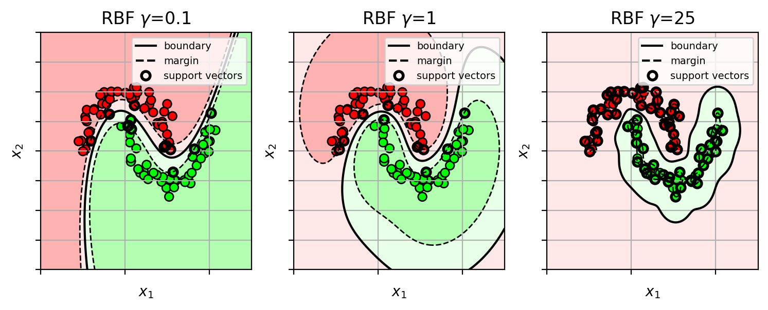
Kernel SVM with RBF kernel

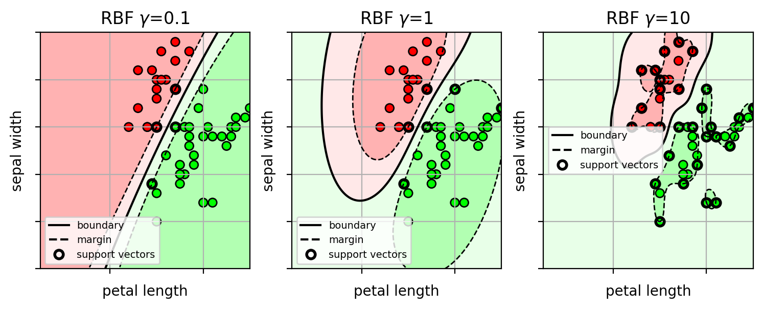
  • try different $\gamma$
    • each $\gamma$ yields different levels of smoothness of the decision boundary
1
2
3
4
5
6
7
# fit SVM (RBF)
gammas = [0.1, 1, 25]

clf = {}
for i in gammas:
clf[i] = svm.SVC(kernel='rbf', gamma=i, C=1000)
clf[i].fit(X3, Y3)
1
2
3
4
5
6
7
8
9
10
11
12
13
14
15
axbox = [-2, 3, -2, 2]

rbfsvmfig = plt.figure(figsize=(9,3))

for i,x in enumerate(gammas):
clfx = clf[x]
plt.subplot(1,3,i+1)

plot_posterior_svm(clfx, axbox, X3)
plt.scatter(X3[:,0], X3[:,1], c=Y3, cmap=mycmap, edgecolors='k')
plt.xlabel('$x_1$'); plt.ylabel('$x_2$')
plt.gca().xaxis.set_ticklabels([])
plt.gca().yaxis.set_ticklabels([])
plt.title('RBF $\gamma$=' + str(x))
plt.close()
1
rbfsvmfig

png

Example on Iris data

  • Large $\gamma$ yields a complicated wiggly decision boundary.
1
2
3
4
5
6
7
8
9
# load iris data each row is (petal length, sepal width, class)
from sklearn.datasets import load_iris

irisdata = load_iris()

X = irisdata.data[:100,0:2] # the first two columns are features (petal length, sepal width)
Y = irisdata.target[:100] # the third column is the class label (versicolor=1, virginica=2)

print(X.shape)
(100, 2)
1
2
3
4
5
6
7
# randomly split data into 50% train and 50% test set
trainX, testX, trainY, testY = \
model_selection.train_test_split(X, Y,
train_size=0.5, test_size=0.5, random_state=4487)

print(trainX.shape)
print(testX.shape)
(50, 2)
(50, 2)
1
2
3
4
5
6
7
8
9
10
11
12
13
14
15
16
17
18
19
# fit SVM (RBF)
gammas = [0.1, 1, 10]

clf = {}
for i in gammas:
clf[i] = svm.SVC(kernel='rbf', gamma=i, C=100)
clf[i].fit(trainX, trainY)

irbffig = plt.figure(figsize=(9,3))
axbox = [2.5, 7, 1.5, 4]
for i,x in enumerate(gammas):
plt.subplot(1,3,i+1)
plot_posterior_svm(clf[x], axbox, trainX)
plt.scatter(trainX[:,0],trainX[:,1],c=trainY, cmap=mycmap, edgecolors='k')
plt.xlabel('petal length'); plt.ylabel('sepal width')
plt.gca().xaxis.set_ticklabels([])
plt.gca().yaxis.set_ticklabels([])
plt.title('RBF $\gamma$=' + str(x))
plt.close()
1
irbffig

png

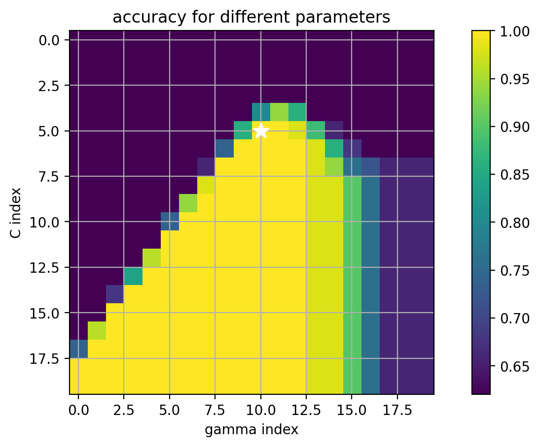
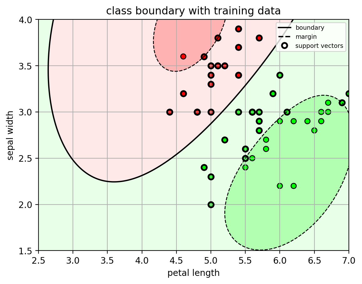
How to select the best kernel parameters?

  • use cross-validation over possible kernel parameter ($\gamma$) and SVM $C$ parameter
    • if a lot of parameters, can be computationally expensive!
1
2
3
4
5
6
7
8
9
10
11
12
13
14
15
# setup the list of parameters to try
paramgrid = {'C': logspace(-2,3,20),
'gamma': logspace(-4,3,20) }

print(paramgrid)

# setup the cross-validation object
# pass the SVM object w/ rbf kernel, parameter grid, and number of CV folds
svmcv = model_selection.GridSearchCV(svm.SVC(kernel='rbf'), paramgrid, cv=5,
n_jobs=-1, verbose=True)

# run cross-validation (train for each split)
svmcv.fit(trainX, trainY);

print("best params:", svmcv.best_params_)
{'C': array([1.00000000e-02, 1.83298071e-02, 3.35981829e-02, 6.15848211e-02,
       1.12883789e-01, 2.06913808e-01, 3.79269019e-01, 6.95192796e-01,
       1.27427499e+00, 2.33572147e+00, 4.28133240e+00, 7.84759970e+00,
       1.43844989e+01, 2.63665090e+01, 4.83293024e+01, 8.85866790e+01,
       1.62377674e+02, 2.97635144e+02, 5.45559478e+02, 1.00000000e+03]), 'gamma': array([1.00000000e-04, 2.33572147e-04, 5.45559478e-04, 1.27427499e-03,
       2.97635144e-03, 6.95192796e-03, 1.62377674e-02, 3.79269019e-02,
       8.85866790e-02, 2.06913808e-01, 4.83293024e-01, 1.12883789e+00,
       2.63665090e+00, 6.15848211e+00, 1.43844989e+01, 3.35981829e+01,
       7.84759970e+01, 1.83298071e+02, 4.28133240e+02, 1.00000000e+03])}
Fitting 5 folds for each of 400 candidates, totalling 2000 fits
best params: {'C': 0.20691380811147891, 'gamma': 0.4832930238571752}
1
2
3
4
# show the test error for the first 25 parameter sets
N = 25
for m,p in zip(svmcv.cv_results_['mean_test_score'][0:N], svmcv.cv_results_['params'][0:N]):
print("mean={:.4f} {}".format(m,p))
mean=0.6200 {'C': 0.01, 'gamma': 0.0001}
mean=0.6200 {'C': 0.01, 'gamma': 0.00023357214690901214}
mean=0.6200 {'C': 0.01, 'gamma': 0.000545559478116852}
mean=0.6200 {'C': 0.01, 'gamma': 0.0012742749857031334}
mean=0.6200 {'C': 0.01, 'gamma': 0.002976351441631319}
mean=0.6200 {'C': 0.01, 'gamma': 0.0069519279617756054}
mean=0.6200 {'C': 0.01, 'gamma': 0.01623776739188721}
mean=0.6200 {'C': 0.01, 'gamma': 0.0379269019073225}
mean=0.6200 {'C': 0.01, 'gamma': 0.08858667904100823}
mean=0.6200 {'C': 0.01, 'gamma': 0.2069138081114788}
mean=0.6200 {'C': 0.01, 'gamma': 0.4832930238571752}
mean=0.6200 {'C': 0.01, 'gamma': 1.1288378916846884}
mean=0.6200 {'C': 0.01, 'gamma': 2.6366508987303554}
mean=0.6200 {'C': 0.01, 'gamma': 6.1584821106602545}
mean=0.6200 {'C': 0.01, 'gamma': 14.38449888287663}
mean=0.6200 {'C': 0.01, 'gamma': 33.59818286283781}
mean=0.6200 {'C': 0.01, 'gamma': 78.47599703514607}
mean=0.6200 {'C': 0.01, 'gamma': 183.29807108324337}
mean=0.6200 {'C': 0.01, 'gamma': 428.1332398719387}
mean=0.6200 {'C': 0.01, 'gamma': 1000.0}
mean=0.6200 {'C': 0.018329807108324356, 'gamma': 0.0001}
mean=0.6200 {'C': 0.018329807108324356, 'gamma': 0.00023357214690901214}
mean=0.6200 {'C': 0.018329807108324356, 'gamma': 0.000545559478116852}
mean=0.6200 {'C': 0.018329807108324356, 'gamma': 0.0012742749857031334}
mean=0.6200 {'C': 0.018329807108324356, 'gamma': 0.002976351441631319}
1
2
3
4
5
6
7
8
9
10
11
12
13
14
15
16
17
18
19
def extract_grid_scores(modelcv, paramgrid):
"extract CV scores from GridSearchCV and put into a matrix"
# get parameters
pkeys = list(paramgrid.keys())

# initialize empty score matrix
scoresize = [len(paramgrid[p]) for p in pkeys]
avgscores = zeros(scoresize)

# fill in the matrix with run for each parameter set
for rm,rp in zip(modelcv.cv_results_['mean_test_score'], modelcv.cv_results_['params']):
# get the index into each of the parameter lists
myind = [where(rp[p] == paramgrid[p]) for p in pkeys]
avgscores[tuple(myind)] = rm # put the score

# location of best score
bestind = [where(modelcv.best_params_[p] == paramgrid[p]) for p in pkeys]

return avgscores, pkeys, bestind
1
2
3
4
5
6
7
8
9
10
(avgscores, pnames, bestind) = extract_grid_scores(svmcv, paramgrid)
paramfig = plt.figure()
plt.imshow(avgscores, interpolation='nearest')
plt.plot(bestind[1], bestind[0], '*w', markersize=12)
plt.ylabel(pnames[0] + ' index'); plt.xlabel(pnames[1] + ' index')
plt.grid(True)
plt.title('accuracy for different parameters')
plt.colorbar()
plt.axis('image');
plt.close()
1
paramfig

png

1
2
3
4
5
6
7
# show classifier with training data
plt.figure()
plot_posterior_svm(svmcv.best_estimator_, axbox, trainX)
plt.scatter(trainX[:,0], trainX[:,1], c=trainY, cmap=mycmap, edgecolors='k')
plt.xlabel('petal length'); plt.ylabel('sepal width')
plt.title('class boundary with training data');
plt.show()

png

1
2
3
4
5
6
# predict from the model
predY = svmcv.predict(testX)

# calculate accuracy
acc = metrics.accuracy_score(testY, predY)
print("test accuracy =", acc)
test accuracy = 0.98

Custom kernel function

  • we can use any kernel function, as long as it is positive semi-definite:
      1. it can be written as an inner-product of a feature transformation: $k(\mathbf{x}_1,\mathbf{x}_2) = \langle \Phi(\mathbf{x}_1), \Phi(\mathbf{x}_2) \rangle$.
      1. for all possible datasets $\mathbf{X} = {\mathbf{x}_1, \cdots \mathbf{x}_N}$ of all possible sizes $N$, the kernel matrix $K=[k(\mathbf{x}_i,\mathbf{x}j)]{i,j}$ is a positive definite matrix.
      • $\mathbf{K}$ is a positive semi-definite matrix iff $\mathbf{z}^T\mathbf{K}\mathbf{z} \geq 0, \forall \mathbf{z}$
  • in sklearn, pass a callable function as the kernel parameter.

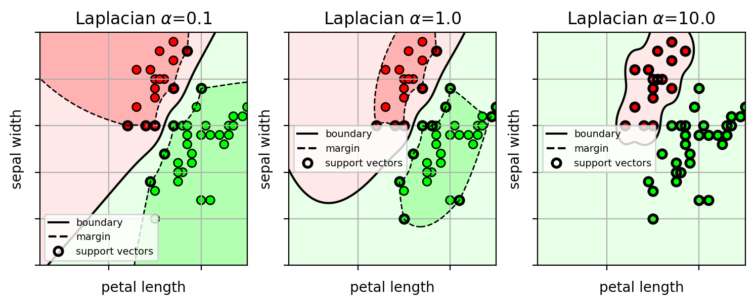
Example: Laplacian kernel

  • $k(\mathbf{x}_1,\mathbf{x}_2) = \exp(-\alpha ||\mathbf{x}_1 - \mathbf{x}_2||)$
1
2
3
4
5
6
7
8
9
10
11
12
13
from scipy import spatial

# create a custom kernel function
# Laplacian kernel: exp( -alpha*||x1-x2|| )
def mykernel(X1, X2, alpha=1.0):
# X1,X2 are (N1 x d) and (N2 x d) matrices of N1 and N2 d-dim vectors
# alpha is the hyperparameter

# compute pairwise euclidean distance
D = spatial.distance.cdist(X1, X2, metric='euclidean')

# return the kernel matrix
return exp(-alpha*D)
1
2
3
4
5
6
7
8
9
10
alphas = [0.1, 1., 10.]

clf = {}
for i in alphas:
# make a temporary kernel function with the selected alpha value
tmpkern = lambda X1,X2,alpha=i: mykernel(X1,X2,alpha=alpha)

# create the SVM with custom kernel function
clf[i] = svm.SVC(kernel=tmpkern, C=100)
clf[i].fit(trainX, trainY)
1
2
3
4
5
6
7
8
9
10
11
ilapfig = plt.figure(figsize=(9,3))
axbox = [2.5, 7, 1.5, 4]
for i,x in enumerate(alphas):
plt.subplot(1,3,i+1)
plot_posterior_svm(clf[x], axbox, trainX)
plt.scatter(trainX[:,0],trainX[:,1],c=trainY, cmap=mycmap, edgecolors='k')
plt.xlabel('petal length'); plt.ylabel('sepal width')
plt.gca().xaxis.set_ticklabels([])
plt.gca().yaxis.set_ticklabels([])
plt.title('Laplacian $\\alpha$=' + str(x))
plt.close()
1
ilapfig

png

Kernel SVM Summary

  • Kernel Classifier:

    • Kernel function defines the shape of the non-linear decision boundary.
      • implicitly transforms input feature into high-dimensional space.
      • uses linear classifier in high-dim space.
      • the decision boundary is non-linear in the original input space.
  • Training:

    • Maximize the margin of the training data.
      • i.e., maximize the separation between the points and the decision boundary.
    • Use cross-validation to pick the hyperparameter $C$ and the kernel hyperparameters.
  • Advantages:

    • non-linear decision boundary for more complex classification problems
    • some intuition from the type of kernel function used.
    • kernel function can also be used to do non-vector data.
  • Disadvantages:

    • sensitive to the kernel function used.
    • sensitive to the $C$ and kernel hyperparameters.
    • computationally expensive to do cross-validation.
    • need to calculate the kernel matrix
      • $N^2$ terms where $N$ is the size of the training set
      • for large $N$, uses a large amount of memory and computation.

Kernels on other types of data

  • Histograms: $\mathbf{x} = [x_1,\cdots, x_d]$, $x_i$ is a bin value.

    • Bhattacharyya: $$k(\mathbf{x},\mathbf{x}’) = \sum_{i=1}^d \sqrt{x_i x’_i}$$
    • histogram intersection: $$k(\mathbf{x},\mathbf{x}’) = \sum_i \min(x_i, x_i’)$$
    • $\chi^2$-RBF: $$k(\mathbf{x},\mathbf{x}’) = e^{-\gamma \chi^2(\mathbf{x},\mathbf{x}’)}$$
      • $\gamma$ is a inverse bandwidth parameter
      • $\chi^2$ distance: $\chi^2(\mathbf{x},\mathbf{x}’) = \sum_{i=1}^d\frac{(x_i-x’_i)^2}{\tfrac{1}{2}(x_i+x’_i)}$
  • Strings: $\mathbf{x}$ = “….” (strings can be different sizes)
    $$k(\mathbf{x},\mathbf{x}’) = \sum_{s} w_s \phi_s(\mathbf{x})\phi_s(\mathbf{x}’)$$

    • $\phi_s(\mathbf{x})$ is the number of times substring $s$ appears in $\mathbf{x}$.
    • $w_s>0$ is a weight.
  • Sets: $\mathbf{X} = {\mathbf{x}_1,\cdots, \mathbf{x}_n}$ (sets can be different sizes)

    • intersection kernel: $$k(\mathbf{X},\mathbf{X}’) = 2^{|\mathbf{X}\cap \mathbf{X}’|}$$
      • $|\mathbf{X}\cap \mathbf{X}’|$ = number of common elements.